PIC microcontrollers sport a number of useful peripheral devices, but some appear to lurk in the background, not getting the attention they deserve. Or maybe it’s just they seem so complicated that the newcomer shies away, not knowing how to begin. The Capture/Compare/Pulse Width Modulation unit (called CCP from now on) is just such a module. And yet it’s so handy, that it’s a shame not to learn how to use it early on.
As the full name implies, the CCP module has been designed to handle three different but vaguely related applications. This tutorial focuses exclusively on the capture aspect. Its primary purpose is to accurately measure the period or duty cycle of an incoming pulse wave. Why might that be useful? There are several interesting situations that come to mind at once. For instance, some outboard devices have been specifically designed to communicate by modulating the duty cycle of a pulse wave. Handheld IR remote control units and the popular DHT22 humidity/temperature sensor are good examples. Another possibility is making pushbutton switches intelligent: pressing momentarily means one thing while pressing-and-holding means another. Maybe an automated camera should only snap pictures if someone or something is lingering on a spot for at least a specified duration. Or how about designing your own system to communicate using pulse-code modulation across a single line? This is also possible with the CCP module operating in capture mode. Just in general, any time you are sensing events that convey meaning according to how long or how fast they occur, the capture module is the helper to call upon. Let’s see how it works.
Overview of the Capture Process
Most PIC microcontrollers contain at least one CCP unit. To keep this tutorial specific, I’ll focus on the common and inexpensive PIC16F88, but bear in mind that the module works similarly in other chips. Let’s consider how it’s been implemented in broad strokes first.
Refer to the figure below which depicts the functional arrangement of the capture module.
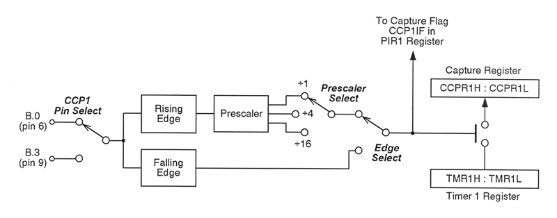
Running in the background is a timer, really just a 16-bit binary counter that keeps chugging away from 0 on up to 65535, rolling over to 0 and continuing likewise in perpetuity. This is denoted Timer1 by the PIC manufacturer. It may be clocked in several different ways, but for now just assume that the system clock of the microcontroller is stepping it along. At any given moment, the two bytes, TMR1H and TMR1L, concatenated to form a word, indicate the current value of Timer1. Let it keep running for the moment, and turn your attention to the left side of the figure.
An external signal is applied to either port line B.0 or B.3. This may be a single pulse if you’re simply measuring the on-time of a switch or a sensor, or could be an ongoing pulse train, if you’re wanting to determine frequency (which is nothing more than the reciprocal of the period). Which port line to be used is determined when the PIC is flashed (programmed). This pin is then denoted CCP1 and devoted exclusively as the input to the CCP module from then on. Observe that this is established by the configuration bits of the chip (what some people call fuses) and doesn’t change once the chip has been flashed.
Jump ahead a little in the figure and notice the edge select switch. Your program can decide whether to sense either rising edges or falling edges. Additionally, in the case of the former choice, you may also have the chip react to every rising edge, every fourth, or every sixteenth. Think of this as a prescaler to slow things down.
Remember, that timer we left a moment ago is still counting away. But whenever an edge event occurs (whichever you selected in the previous step), the current value of the timer is latched into the capture register made up of the two bytes CCPR1H and CCPR1L. Thus, you have a record of how many increments Timer1 has made since the last edge event. Because the timer runs at a predictable frequency, we then know exactly how much time has been consumed. If you’d like, think of this as one of the those elapsed-time stopwatches used in sporting events.
With the principle of operation out of the way, we can now get serious about the nuts and bolts of actually setting things up. Unlike the PIC data sheet which throws you into the deep end of the pool, I’ve broken things up into logical units to be easily assimilated. Tackling the details becomes so much more straightforward.
Setting up Capture Mode
As a basic road map, here’s what needs to be done in order to get the capture module up and running:
- establish which pin is CCP1 and make it an input
- set the rate at which the timer operates
- start the timer counting
- set which type of edge event is desired, rising or falling
- set the prescaler for rising edges, if needed
- monitor the results directly or use interrupts

Additionally, your program proper should also designate that this is an input port line. (Remember, it’s the pin to which you apply the external signal being monitored.) If you’re an assembly language aficionado and get off on bit-twiddling, then you already know how to handle this and what’s to come. But to the rest of you, sit tight and in a moment I’ll show you how to make these adjustments easily in the PIC Micro Pascal.
The figure below shows the T1CON register and the bits to be manipulated to get the timer up and running.

Generally, you’ll want the timer to be stepped along by the microcontroller’s system clock. Actually, due to the way microcontrollers read and process individual instructions, the timer is being pulsed at a rate one-quarter that of the clock frequency. So, for example, with the PIC16F88 operating under an 8MHz clock (use a crystal or resonator for best accuracy), Timer1 runs at 2MHz, meaning that it increments once every 0.5 microseconds. This rate can be modified by way of the Timer1 prescaler as indicated in the above figure. Finally, setting the bit TMR1ON revs up the timer which will take care of itself from then on, running continually in the background.
The next figure shows how to choose the capture module edge type and optional prescaler. This is handled by register CCP1CON.

How to Read the Captured Events
If you look back to the block diagram we started with, above, you’ll notice that every time a capture is made, the flag CCP1IF is set. This bit is found in the register entitled PIR1. While there’s certainly no reason why your program couldn’t monitor this from within an endless loop, it’s much more efficient to employ interrupts. In a nutshell, your main program can do whatever it normally should be doing, but when a capture is made, it stops long enough to fetch the new number in CCP1H:CCP1L before returning to the main action. Rather than trying to explain everything about all interrupts, the following figure zeros in exclusively on what you need to know when working with the capture module.

Let’s pull this all together and see the pieces that make up some actual working code in the PIC Micro Pascal language.
Okay, your first step is to set CCP1 and make it an input. As for the former, can you spot it in these configuration settings (which occur toward the start of your program)?
{$CONFIG BOREN = OFF,
CCPMX = RB0,
CP = OFF,
CPD = OFF,
DEBUG = OFF,
FOSC = HS,
LVP = OFF,
MCLRE = OFF,
PWRTE = OFF,
WDTE = OFF,
WRT = OFF}
Then, in the program proper, this will take care of the latter:
CapDDR := 1; // make input on pin 6
assuming the following were defined in the variable section of your program:
CapPin : boolean @ PortB.RB0;
CapDDR : boolean @ GET_TRIS(CapPin);
Then it’s a snap to adjust Timer1 and get it running in the code with:
CCP1CON := [CCP1M = 0b0101]; // capture rising edge
T1CON := [T1CKPS = 0b10, // prescaler = 4
TMR1CS = 0, // clock = oscillator/4
TMR1ON = 1]; // turn on the timer
Last, we turn on the interrupt business with:
PIE1 := [CCP1IE]; // enable capture interrupt
INTCON := [GIE, PEIE]; // turn on interrupts
That’s it! The timer is running, port line B.0 is monitoring the incoming pulse wave, and every time the signal starts afresh with a new rising edge, the current timer value is stored in the capture register and an interrupt occurs. The interrupt routine then processes the information as desired.
Speaking of which, let’s conclude with two experiments illustrating the most common applications of the capture module. Take a moment to actually carry these out, for once you’ve done so, you’ll really have a grasp of the details.
Measuring Period
The following figure shows the schematic for both of these experiments.

You can patch it up in minutes on a breadboard. Next, download the source code:
In Experiment #1 we’re going to determine the period of an incoming pulse train. Program the PIC from the source code you just downloaded, then build up the circuit in the schematic, above. Use an 8 MHz resonator. You may eliminate the potentiometer, which is unneeded here. Finally, apply a source of pulse waves to the CCP1 pin, making sure that it has an amplitude of 0 to +5V to match the PIC. I used a homemade function generator when I ran the exercise.
Fire things up and you’ll see the period of the incoming signal displayed on the LCD, in microseconds. Vary the frequency of your pulse source from 15 Hz on up and note the results.
So how does it work? Check out the interrupt routine and all becomes clear:
current := CCPR1 - mark; // the current period
mark := CCPR1; // mark where we left off
PIR1 := [CCP1IF = 0] // clear capture flag
A simple subtraction is all it takes. In particular, the previous value of the timer is subtracted from the current value just captured, and since Timer1 is effectively clocking along at 1 tick per microsecond, that difference gives a direct period measurement in microseconds. Simple!
Here's a pic of it in operation:

Measuring Duty Cycle
Measuring the duty cycle of an incoming pulse wave is only slightly more involved. For this exercise, you’ll build the circuit in the schematic twice, one to serve as a transmitter and the other to act as the receiver. This time, use 20 MHz resonators. You may eliminate the pot on the receiver.
The transmitter outputs a pulse wave whose duty cycle is modulated under control of the potentiometer. This waveform appears on CCP1, which obviously is an output since we’re transmitting. (See the previous PIC Tutorial to learn how PWM works).
The output then connects to the CCP1 input of the receiver. Varying the duty cycle of the first is then reported on the LCD display of the second. We are literally conveying a broad range of numbers along a single wire by means of a pulse duty cycle. Here's what it looks like:

The steps involved here are quite interesting. First, the receiver is set to react to a rising edge. This would be the start of the pulse. But then the capture module is changed to respond to a falling edge, indicating the end of the on-time. Finally, the next rising edge signals the conclusion of the entire cycle. In short, with a couple subtractions we’ve found the on-time and the length of the entire cycle. Dividing the latter into the former yields the duty cycle when interpreted as a percentage. It’s a pretty cool demonstration, so be sure to study the source code which is heavily commented.
Note that trying to detect a duty cycle less than 2% or more than 98% is tricky without some serious recoding, since the interrupts occur so quickly in the short regions of the waveform. However, for all values between these two extremes, the transmission is quite reliable in the present experiment.
With that, we come to the end of this tutorial, but certainly not the end of what can be accomplished with the capture module. And, best of all, you should be in good shape to tackle the complete data sheet for the PIC and take on even more advanced applications.
Next Tutorial: The Compare Module
No comments:
Post a Comment